%pip install -Uqq plotly seabornNote: you may need to restart the kernel to use updated packages.In the ever-evolving realm of machine learning and image processing, one dataset has stood the test of time as a benchmark for countless algorithms and models: the MNIST dataset. Short for the Modified National Institute of Standards and Technology database, MNIST is a treasure trove of handwritten digits, ranging from 0 to 9, encapsulated within a repository of 70,000 grayscale images. In this blog post, we will delve into the intricacies of MNIST, exploring its significance, structure, and applications.
Before properly starting, I’ll be importing the necessary libraries and also loading our data.
%pip install -Uqq plotly seabornNote: you may need to restart the kernel to use updated packages.from torch.utils.data import Dataset, DataLoader
from sklearn.metrics import confusion_matrix
import matplotlib.pyplot as plt
import torch.nn.functional as F
import plotly.express as px
from torch.optim import SGD
from tqdm import tqdm
import seaborn as sns
import torch.nn as nn
import numpy as np
import torchvision
import torch
%matplotlib inline
device = 'cuda' if torch.cuda.is_available() else 'cpu'
print(f'Using {str.upper(device)} device 🌟')
x, y = torch.load('./MNIST/processed/training.pt')
print(x.shape, y.shape)Using CUDA device 🌟
torch.Size([60000, 28, 28]) torch.Size([60000])We can then visualize a sample:
fig = plt.figure(figsize=(4, 3.5))

def show_number(i: int = 0):
    plt.imshow(x[i].numpy(), cmap='Blues')
    plt.title(f'The number is {y[i].numpy()}')
    plt.colorbar()

    plt.show()

show_number(20)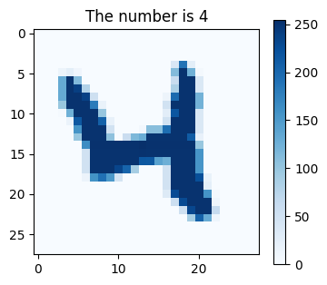
A next step is using One Hot Encoder to transform categorical data into numerical data. In this case, representing the digits 0-9 it’ll allow each label to be represented as a binary vector that is all 0 except the index of the integer (label) itself that’d be marked as 1.
# Performing a test before properly apply to our dataset

original_y = torch.tensor([2, 4, 3, 0, 1])
new_y = F.one_hot(original_y)
new_y
tensor([[0, 0, 1, 0, 0],
[0, 0, 0, 0, 1],
[0, 0, 0, 1, 0],
[1, 0, 0, 0, 0],
[0, 1, 0, 0, 0]])# Applying in the MNIST data
new_y = F.one_hot(y, num_classes=10)
y.reshape(-1, 1).shape[-1], new_y.shape[-1] # Expected (1, 10)(1, 10)This is another important step as a class is used to represent a collection of data that can be used for training a model. It is an abstract class that can be inherited to create a custom dataset that can be used to load and manipulate sets containing data in many forms.
class CTDataset(Dataset):
    def __init__(self, filepath):
        self.x, self.y = torch.load(filepath)
        self.x = self.x / 255.
        self.y = F.one_hot(self.y, num_classes=10).to(float)

    def __len__(self):
        return self.x.shape[0]

    def __getitem__(self, ix):
        return self.x[ix], self.y[ix]

train_dataset = CTDataset('./MNIST/processed/training.pt')
test_dataset = CTDataset('./MNIST/processed/test.pt')Here’s the time when we create the dataloader objects. These are important components of Deep Learning pipelines that help to load and preprocess data for training. They are used to handle large datasets and perform data ugmentation, shuffling, and other preprocessing tasks.
They are importat for some reasons including: Standardisation, Efficiency and Flexibility.
train_dataloader = DataLoader(train_dataset, batch_size=5)

for x, y in train_dataloader:
    x = x.to(device)
    y = y.to(device)
    print(x.shape)
    print(y.shape)
    break

print(f'\n{len(train_dataloader)}')
torch.Size([5, 28, 28])
torch.Size([5, 10])
12000Now, Cross-entropy loss is a widely used loss function in classification tasks. It has several advantages that make it popular, including:
L = nn.CrossEntropyLoss().to(device)
LCrossEntropyLoss()As we’re approaching this problem using Deep Learning, a neural network is important to keep it functional - so, here I declare the network for this classifier:
class DigitsClassifier(nn.Module):
    def __init__(self):
        super().__init__()
        self.Matrix1 = nn.Linear(28**2,100)
        self.Matrix2 = nn.Linear(100,50)
        self.Matrix3 = nn.Linear(50,10)
        self.R = nn.ReLU()

    def forward(self,x):
        x = x.view(-1,28**2)
        x = self.R(self.Matrix1(x))
        x = self.R(self.Matrix2(x))
        x = self.Matrix3(x)

        return x.squeeze()

        # output = x.squeeze()

        # return output.argmax(axis = 1)

model = DigitsClassifier().to(device)
model
DigitsClassifier(
(Matrix1): Linear(in_features=784, out_features=100, bias=True)
(Matrix2): Linear(in_features=100, out_features=50, bias=True)
(Matrix3): Linear(in_features=50, out_features=10, bias=True)
(R): ReLU()
)xs, ys = train_dataset[0:5]
model(xs.to(device))tensor([[-0.0759, -0.0578, -0.0325, 0.1515, -0.0489, -0.0079, -0.0817, 0.1410,
-0.0657, -0.0913],
[-0.0584, -0.0314, -0.0718, 0.1930, -0.0209, -0.0429, -0.0243, 0.1449,
-0.0411, -0.0707],
[-0.0568, -0.0475, -0.0563, 0.1828, -0.0044, -0.0150, -0.0350, 0.1090,
-0.0087, -0.0581],
[-0.0622, -0.0535, -0.0551, 0.1234, -0.0365, -0.0321, -0.0423, 0.1067,
-0.0618, -0.0971],
[-0.0458, -0.0897, -0.0495, 0.1648, 0.0038, -0.0291, -0.0159, 0.0708,
-0.0066, -0.0851]], device='cuda:0', grad_fn=<SqueezeBackward0>)L(model(xs.to(device)), ys.to(device))tensor(2.3381, device='cuda:0', dtype=torch.float64, grad_fn=<DivBackward1>)Another essential part of a machine learning process is training. It involves optimizing the parameters of a model to minimize the difference between the predicted output and the true output. In the given code, I’ll be defining a function to do it for us that takes as input a data loader, a model, and the number of epochs.
During training, the function iterates over the data loader and updates the model parameters using backpropagation and gradient descent. The loss and epoch data are recorded for each iteration, which will be used to visualize the training progress and evaluate the performance.
def train_model(
    dataloader: torch.utils.data.dataloader.DataLoader,
    model: DigitsClassifier,
    n_epochs: int = 30) -> tuple[np.ndarray, np.ndarray]:

    optimizer = SGD(model.parameters(), lr=1e-2)
    L = nn.CrossEntropyLoss()

    losses = []
    epochs = []

    for epoch in range(n_epochs):
        print(f'Epoch: {epoch + 1}/{n_epochs} | Loss: {np.mean(losses)}')
        N = len(dataloader)

        for i, (x, y) in enumerate(dataloader):
            x = x.to(device)
            y = y.to(device)

            optimizer.zero_grad()
            loss_value = L(model(x), y)

            if loss_value > torch.max(y).item():
                torch.save(model.state_dict(), './MNIST/models/mnist_model.pth')

            loss_value.backward()
            optimizer.step()

            epochs.append(epoch + i / N)
            losses.append(loss_value.item())

    return np.array(epochs), np.array(losses)

epoch_data, loss_data = train_model(train_dataloader, model)
/usr/local/lib/python3.9/dist-packages/numpy/core/fromnumeric.py:3432: RuntimeWarning: Mean of empty slice.
return _methods._mean(a, axis=axis, dtype=dtype,
/usr/local/lib/python3.9/dist-packages/numpy/core/_methods.py:190: RuntimeWarning: invalid value encountered in double_scalars
ret = ret.dtype.type(ret / rcount)Epoch: 1/30 | Loss: nan
Epoch: 2/30 | Loss: 0.444299907778694
Epoch: 3/30 | Loss: 0.30499113273745887
Epoch: 4/30 | Loss: 0.2411346833651296
Epoch: 5/30 | Loss: 0.20264087833581762
Epoch: 6/30 | Loss: 0.17611513000308468
Epoch: 7/30 | Loss: 0.15636798159883528
Epoch: 8/30 | Loss: 0.1409401671701855
Epoch: 9/30 | Loss: 0.1283711091479482
Epoch: 10/30 | Loss: 0.1178500554705612
Epoch: 11/30 | Loss: 0.10884905771381158
Epoch: 12/30 | Loss: 0.10104153238275904
Epoch: 13/30 | Loss: 0.09419568914679677
Epoch: 14/30 | Loss: 0.08814844876493146
Epoch: 15/30 | Loss: 0.08278729691344265
Epoch: 16/30 | Loss: 0.07798079398823612
Epoch: 17/30 | Loss: 0.073632377445332
Epoch: 18/30 | Loss: 0.06971223861976696
Epoch: 19/30 | Loss: 0.06615196071459868
Epoch: 20/30 | Loss: 0.06291801628939395
Epoch: 21/30 | Loss: 0.05995343980754616
Epoch: 22/30 | Loss: 0.057242643725737494
Epoch: 23/30 | Loss: 0.0547542955197936
Epoch: 24/30 | Loss: 0.052467638791425374
Epoch: 25/30 | Loss: 0.050359719916244224
Epoch: 26/30 | Loss: 0.04841136845960758
Epoch: 27/30 | Loss: 0.04660600281967505
Epoch: 28/30 | Loss: 0.04492906776820902
Epoch: 29/30 | Loss: 0.04336751992388834
Epoch: 30/30 | Loss: 0.04190996822760929fig = plt.figure(figsize=(4, 3.5))
plt.plot(epoch_data, loss_data, color='darkblue')
plt.xlabel('Epoch Number')
plt.ylabel('Cross Entropy')
plt.title('Cross Entropy (per batch)')
plt.show()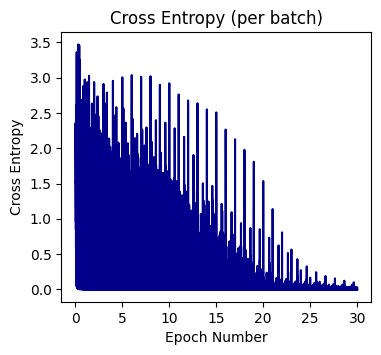
epoch_data_avgd = epoch_data.reshape(20,-1).mean(axis=1)
loss_data_avgd = loss_data.reshape(20,-1).mean(axis=1)

fig = plt.figure(figsize=(4, 3.5))

plt.plot(epoch_data_avgd, loss_data_avgd, 'o--', color='darkblue')
plt.xlabel('Epoch Number')
plt.ylabel('Cross Entropy')
plt.title('Cross Entropy (avgd per epoch)')

plt.show()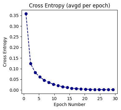
xs, ys = train_dataset[0: 2000]
xs = xs.to(device)
ys = ys.to(device)

yhats = model(xs).argmax(axis = 1)
yhats
tensor([5, 0, 4, ..., 5, 2, 0], device='cuda:0')fig, axes = plt.subplots(3, 4, figsize=(12, 9))
for i in range(12):
row = i // 4
col = i % 4
ax = axes[row, col]
ax.imshow(xs.to('cpu')[i], cmap='Blues')
ax.set_title(f'Predicted Digit: {yhats[i]}')
plt.tight_layout()
plt.show()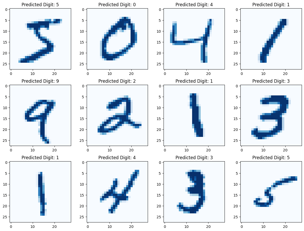
Now it’s time to test our model with unseen data. For this, I’ll be using the test data loader and also plotting the predictions and the confusion matrix.
xs, ys = test_dataset[:2000]
yhats = model(xs.to(device)).argmax(axis = 1)
fig, axes = plt.subplots(3, 4, figsize=(12, 9))
for i in range(12):
row = i // 4
col = i % 4
ax = axes[row, col]
ax.imshow(xs.to('cpu')[i], cmap='Blues')
ax.set_title(f'Predicted Digit: {yhats[i]}')
plt.tight_layout()
plt.show()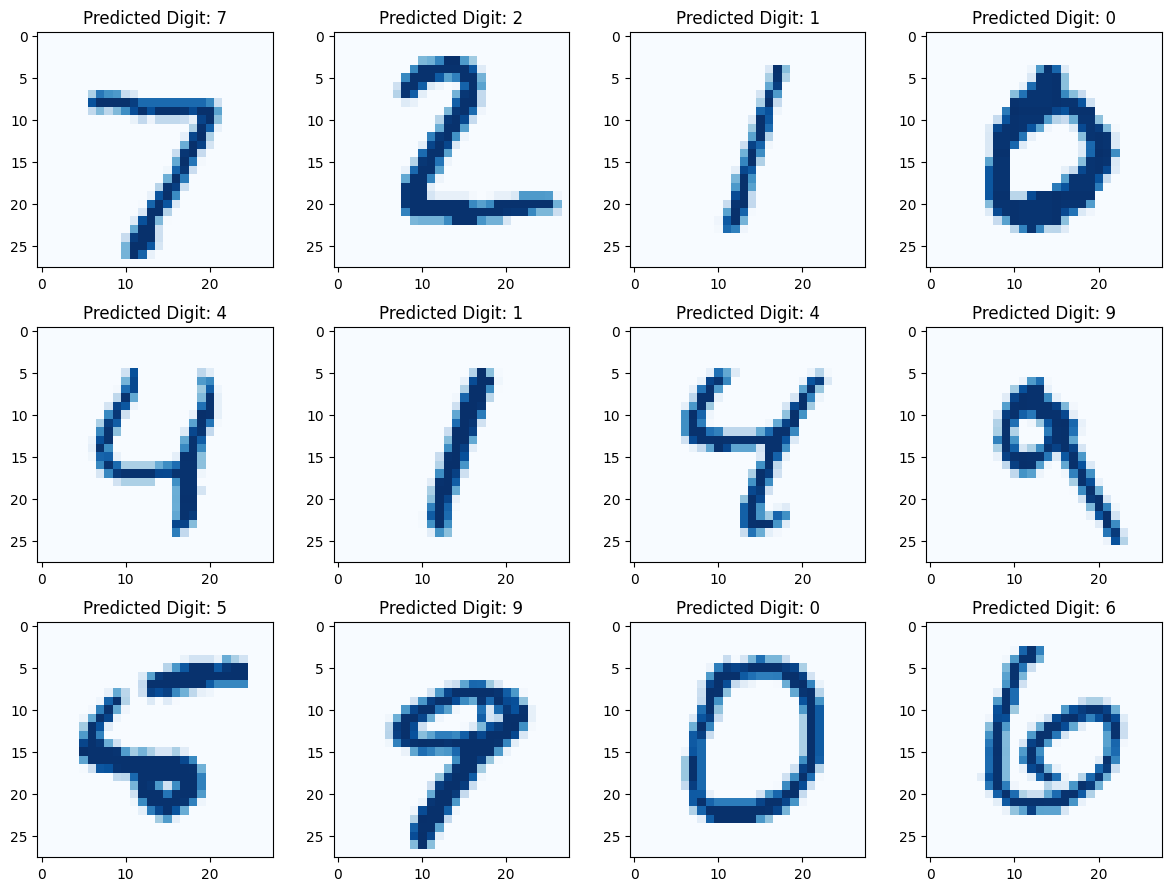
A confusion matrix is an important tool in machine learning that is used to evaluate the performance of a classification model. It is a table that compares the predicted values with the actual values and shows how many predictions are correct and incorrect per class.
images, true = test_dataset[:]
predictions = model(images.to(device)).argmax(axis = 1)
true = torch.argmax(true, dim=1)
scm = confusion_matrix(true.tolist(), predictions.tolist())
scm_normalized = np.round(scm/np.sum(scm, axis=1).reshape(-1, 1), 2)
plt.figure(figsize=(8, 5))
sns.heatmap(
scm_normalized,
cmap='Blues',
annot=True,
cbar_kws={
'orientation': 'vertical'
}
)
plt.xticks(fontsize=12)
plt.yticks(fontsize=12)
plt.title('Confusion Matrix\n', fontsize=18)
plt.xlabel('\nPrediction\n', fontsize=16)
plt.ylabel('\nTrue\n', fontsize=16)
plt.show()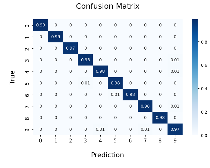
Today, we’ve explored how to develop a solution for the MNIST dataset, and it’s important to note that there are also many other ways to approach this task. We could use TensorFlow instead, apply early stopping techniques, delve deeper into the evaluations, and more. However, we’ve learned how to utilize PyTorch to aid in our deep learning development.
The code developed here is available on my Github.
Thanks for reading, I’ll see you in the next one ⭐