Dive with me into the fascinating role of the Perceptron in shaping AI’s cutting-edge applications and remarkable results.
DEEP LEARNING
DATA SCIENCE
Author
Naomi Lago
Published
September 7, 2023
The Artificial Neural Networks (ANN), inspired by the human brain operation, are inovative computational models and they perform fundamental roles in a variety of field in Computer Science and Artificial Intelligence (AI). They consists of multiple processing units, known as artificial neurons, interconnected to make information processing - and, with the constant advances and the accessibility to Big Data, these networks has been extremely effective when handling complex tasks in Machine Learning.
In this post, I’ll talk about a fundamental concept in this field: the Perceptron. We’ll be exploring its characteristics, fundamentals and applications, despite getting to know its importance in AI. Understand the Perceptron is essential to the comprehension when developing ANN, offering valuable insights about its role in complex problem solvings.
The Perceptron is a concept that was developed by Frank Rosenlatt back in 1958 as a physical analog computer capable of calculating a weighted sum and adapting its weights.
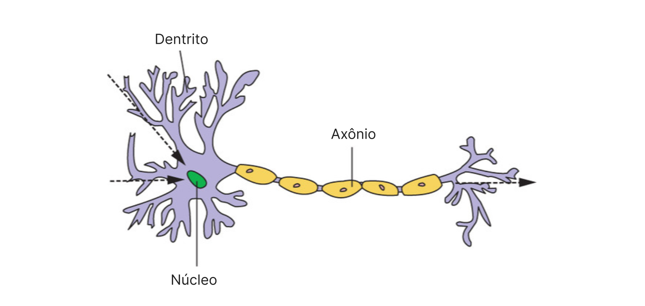
The basis is an approximate imitation of the functioning of a live neuron cell. As electrical signals flow into the cell through dentrites towards the nucleous, an electric charge begins to accumulate. When the cell reaches a certain level of charge, it fire - sending an electrical signal down the axon. However, because dentrites are not all the same, the cell is more “sensitive” to signals through certain dentrites than others, so a smaller amount of signal in those pathways is required to trigger the axon.
Source: Manning Publisher
Indeed, the biology that governs these relationships is beyong the scope of this text, but the key concept to be noted here is how the cell weights the received signals when deciding when to fire. The neuron will dynamically adjust these weights in the decision-making process throughout its life, and in this post, we will mimic this process.
Weight and Bias
Let’s imagine that you are trying to predict the outcome of a badminton game based in various factors such as the wheather, player quality, and coach experience. With a bias and the weights assigned to each factor, a perceptron could be a way to make this decision.
We can think of the weight as the importance we assign to each factor in predictiong the outcome. For example, you can give a higher weight to the weather if you believe it is a crucial factor - since, even though badminton is often played indoors, when played outdoors, wind can have a significant impact on the shuttlecock’s trajectory. In this way, the weight represents the relative relevance of each factor in the decision-making process.
The bias, on the other hand, is a kind of adjustment or tendency we apply to our prediction, regardless of the specific factors involved. Continuing with the example of the badminton game, we can think of bias as the personal inclination we have when making a prediction - even without considering external factors. For instance, if you are a fan of a particular team, you may have a positive bias towards it, meaning that your prediction tends to be more optimistic than that of the others.
These concepts are applied in a perceptron to aid the classification or prediction of outcomes based on different inputs.
Perceptron operation
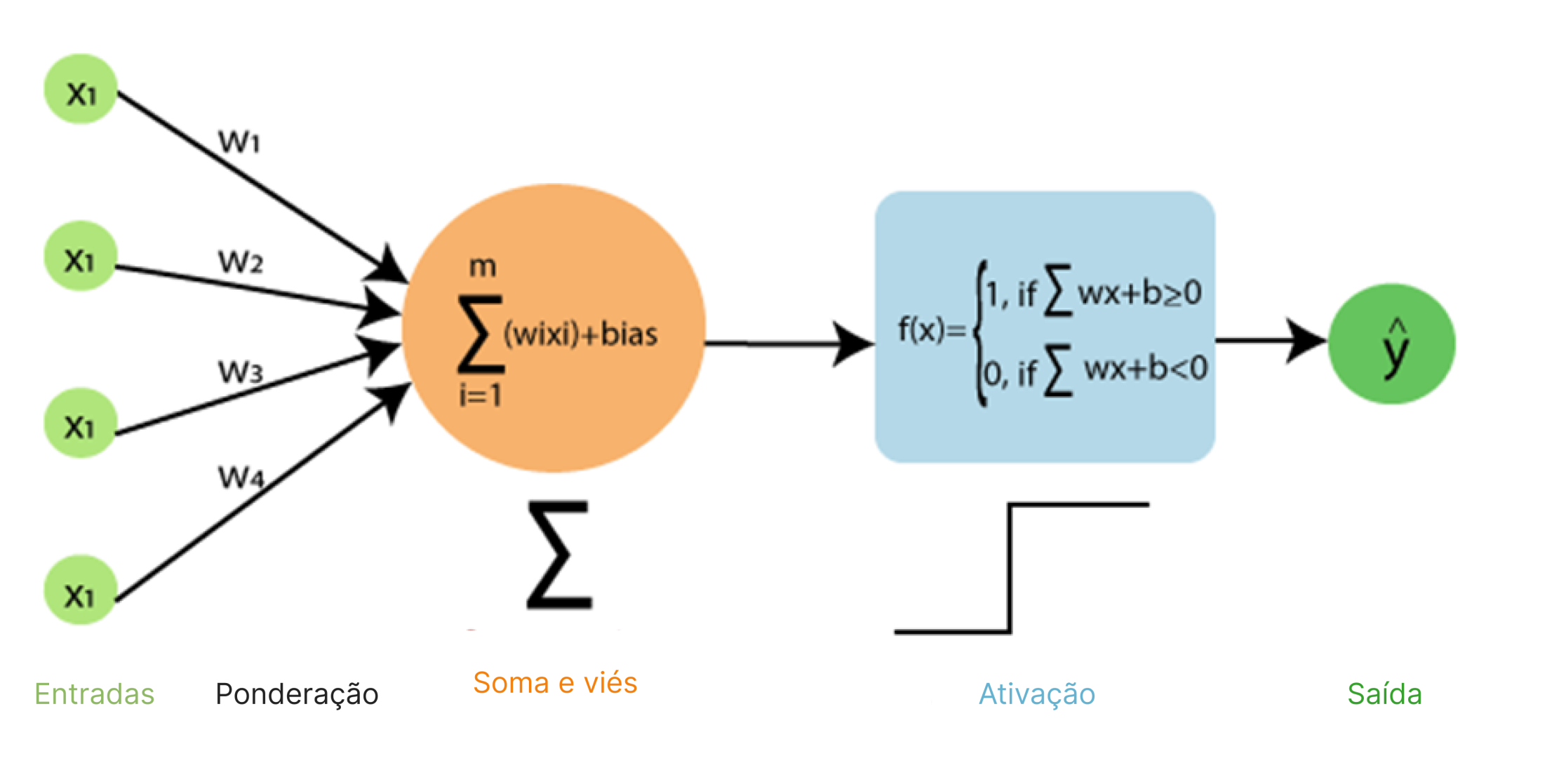
The operation of a Perceptron can be divided into 6 stages, ranging from receiving inputs to the output. Below, we can observe the basic formula and understand each of them.
Source: Nomidl (adapted)
Input: Receives a vector of inputs, representing the attributes or characteristics of the problem at hand.
Weighting: Each input is multiplied by its corresponding weight.
Summation: The weighted values of the inputs are summed.
Bias: The sum value is added to a bias.
Activation: The total value obtained passes through a function that defined the threshold for neuron activation. This function can be binary, returning 0 or 1, or continuous, returning values within a range.
Output: The output is determined by the activation function. Depening on the task at hand, the output can represent a class or a numeric estimate.
During training, the weights are adjusted iteratively based on classification errors or deviations between the output and the desired value. This process of weight adjustment can be performed by algorithms such as the Perceptron or backpropagation.
Implementing a classifier
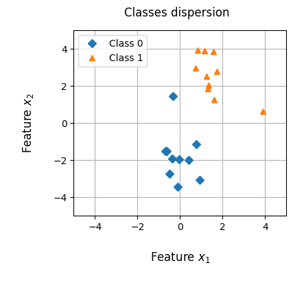
Now, using the concepts we’ve discussed earlier, let’s implement a binary classifier in Python. I’ll follow the hypothetical example of a Badminton match, considering temperature and player experience. Te data has been normalized within a range of -4 to 4, taking into account that neural networks can be sensitive to large values, although this is often scaled down to a smaller range, like -1 to 1.
Below, for reference, I provide the general formula ready to pass through the activation function.
\[b + \sum_{i=0}^{n}x_iw_i\]
Setting up
Let’s start importing the libraries and reading our data using pandas. Below, you can find the code, a sample of 3 records and a table representing the data.
Setting up code
import matplotlib.pyplot as pltfrom loguru import loggerimport pandas as pdimport numpy as np%matplotlib inlineuri ='assets/badminton_data.txt'df = pd.read_csv(uri, sep='\t')df = df.sample(len(df), random_state=20)iflen(df) !=0:print(f'Dataset imported successfully with a shape of {df.shape}')else: logger.error(f'Something went wrong when importing the dataset.')df.sample(3, random_state=10)
Dataset imported successfully with a shape of (20, 3)
temperature
experience
class
12
0.83
3.94
1
8
-0.10
-3.43
0
14
1.14
3.91
1
The temperature is measured in degrees Fahrenheit, the experience in years, and the class refers to the whether the player on the match or not.
Observing the plot and looking at our hypothetical situation, we can see that those with more experience tend to win, for example.
This method is responsible for calculating the weighted sum, adding the bias and applying the activation function. Let’s see how this can be implemented.
Anoter important method for a Perceptron is the update method. The objective here is to adjust the synaptic weights of the model to improve its ability to make correct predictions. The update is performed based on the comparison between the output and the expected value, and one of the most commonly used rules is the Widrow-Hoff rule, known as the Delta rule. To demonstrate its application, I will use a simplified form:
Now that our model is built, let’s move towards finalization by starting the training - which will iterate through the defined number of epochs, making predictions, and updating the parameters to minimize errors.
def training(model, x_values, y_values, epochs):print(f'STARTING THE TRAINING WITH {epochs} EPOCHS')for epoch inrange(epochs): error_count =0for x, y inzip(x_values, y_values): error = model.update(x, y) error_count +=abs(error)print(f'Epoch: {epoch +1} | Errors: {error_count}')print('-'*25)if error_count ==0:breaktraining( model=model, x_values=X_train, y_values=y_train, epochs=5)
Finally, let’s evaluate our model using accuracy - a simple and intuitive measure that indicates the success rate of a model in relation to the expected results. In an ideal and hypothetical world like this problem, we achieved an accuracy of 100%, but it’s important to remember that in real-world data, this value can often fall within a range of 80-90%.
def compute_accuracy(model, x_values, y_values): correct =0.0for x, y inzip(x_values, y_values): prediction = model.forward(x) correct +=int(prediction == y)return correct /len(y_values)training_accuracy = compute_accuracy(model, X_train, y_train)print(f'The training accuracy was {training_accuracy *100}% ⭐')
The training accuracy was 100.0% ⭐
Conclusion
In tis article, we explored the fundamental concept of the Perceptron and its significance in the field of AI. We discussed how it works, covering the steps of weighting, summation, bias, activation, and output. Additionally, we examined the concepts of weight and bias, which play a crucial role in its decision-making process.
Next, we provided a practical implementation of a binary classifier using a Perceptron and Python. We used a hypothetical example of prediction the outcomes of a Badminton match, considering the attributes of temperature and player experience. We demonstrated the process of initialization, forward pass, update, training, and model evaluation.
In conclusion, I state that the Perceptron is a powerful and versatile computational model that can be applied in various fields. Understanding it is essential for the development and application of neural networks, providing valuable insights into machine learning and its ability to solve complex problems.
Thanks for reading, I’ll see you in the next one ⭐